photon (Rendering Architecture Experiment) (2003)

In my CS488 class, right after Semiramis, the final project was one where students created their own assigments, within a structure of guidelines.  I chose to create a simple rendering pipeline, from modelling package to rendering.  I gave this pipeline the (very original) name "photon".

Modelling Aids

As a modelling package, I used Milkshape.  My first two tools were created to help in modelling, because as great as Milkshape was, it was missing a few key features.

To work on the car I wished to model, I required geometry mirroring, something Milkshape did not handle at the time.  To remedy this, I wrote a stand-alone tool called msmirror which looked for specific tags in group names and mirrored geometry right in the .MS3D file.  This tool operated on the command-line, and simply transformed the source file by adding or re-mirroring existing geometry.  This way, I was able to mirror one side of the car to obtain the other.

I also required more sophisticated UV mapping and texture paging functionality than was available.  I thus created a second tool to process .MS3Ds, called msmapper.  This interactive tool allowed me to map and texture page each group within the model individually, changing projection types, etc., and save the results back to the model.  This granted me much finer control over UVs and texture pages than was otherwise available.

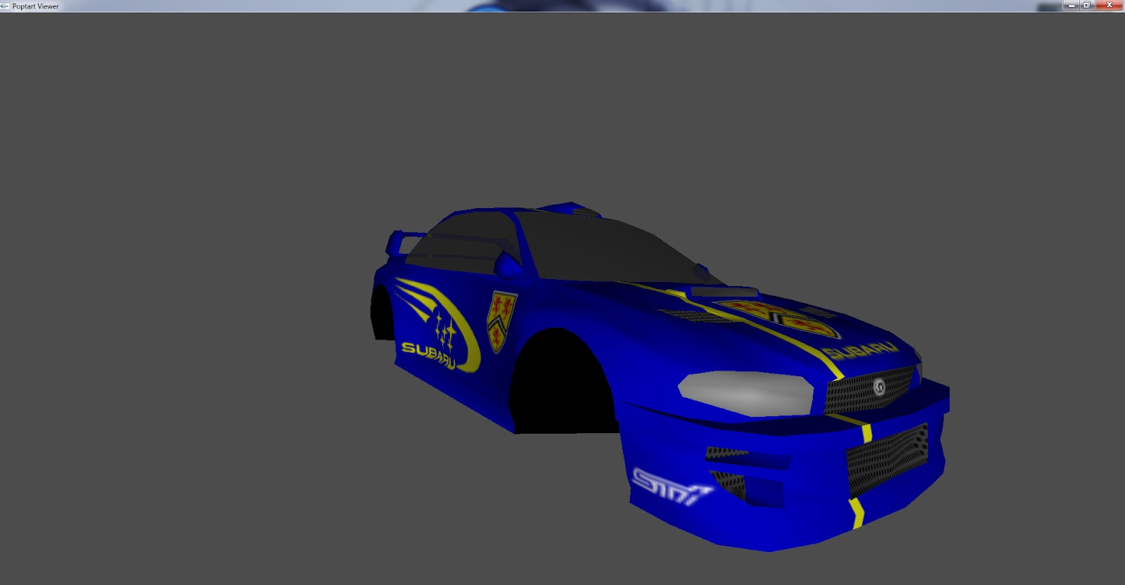
With great pain, I modelled a Subary Impreza WRX STi by pushing vertices, which was great fun and a good learning experience.  The resulting polygon mesh is gross, but hey you have to start somewhere.

I still had no good texture for the wheels, however, when one day I saw a beautiful STi parked outside a restaurant right beside where I lived.  I walked right into the restaurant and went from table to table until I found the owner, from whom I requested permission to photograph the car and its wheels.

Triangle-Batching Tool

Next, I wrote a tool to perform fanning and stripping on my modelled geometry, since on my GeForce 256 those were the fastest primitive types to use.  They cut down both on bandwidth and transformation costs.  (Nowadays different bandwidth limitations and large post-transform vertex caches frequently make it more interesting to use triangle lists instead, but that wasn't the case here.)

My tool used a a few simple heuristics to do its job.  It would begin by first splitting any vertices as required to handle any texturing and normal requirements, since fixed-pipeline OpenGL doesn't support independent indexing for separate attributes.  Next, it would create fans around any vertex used by 8 or more triangles:

Lastly, it would create strips by brute force, using a few heuristics.  It would first examine each of the remaining unbatched triangles and locate the triangles with the lowest number of unbatched neighbours (treating any triangle pair with an edge in common as neighbours):

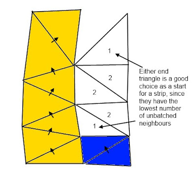
In the set of triangles with the lowest number of neighbours, it would iterate over each triangle's vertices and sum the number of triangles who used that vertex.  It would the prefer triangles for which the sum was lowest:

The goal of this last heuristic was to make the algorithm try to strip "dangling triangles" on the edge of the mesh sooner, because these were more likely to become orphans later down.  Without it, the algorithm frequently picked triangles in the "middle" of the mesh as starting points, which not only left a bunch of orphans on the edges but also sometimes "cut" an arbitrary stripped path from the center of the mesh to its edge, cleaving the space of available triangles for strips to be formed afterwards.  I'm definitely not sure this last heuristic is advantageous in the general case, however - it may just be because of my input data.  I would have needed to try my tool on more data sets to be sure.

Once the set of starting "problem triangles" was known, a simple brute-force search across all edges of the triangles in the starting set was made to find which edge and winding order yielded the longest strip.  This strip was saved and the process was repeated until all triangles were batched.

The quality of the resulting strips and fans depended on the inputs:

Generally pretty crappy stripping, due to wonky input geometry.  Note how the door and windows are a little better since I had an easier time modelling them, and as such the edge topology was much more intelligible.

Great fan and strips for the wheel geometry.

Run-Time Library

Afterwards, the idea was to get this geometry rendering as fast as possible.  I wanted a few simple effects: transparency for the glass and a volumetric lighting effect for the headlights.  (This last effect simply leveraged destination alpha with a special blend mode to lighten the frame buffer only where the dust particles appeared.)

I also included a real-time blurring test, done by rendering many lightly-transparent quads with the same texture, slightly offset from each other:

My goal with this project was to try out a simple method of minimizing graphics pipeline state changes while rendering a scene, since state changes were (and still are) quite expensive.  In order to concentrate on this, I stuck to the OpenGL fixed pipeline model; the scene didn't really require anything programmable anyway, and that axis of exploration was sort of orthogonal to the state change issue.

The idea implemented by photon is simply that each logical object that requires rendering - be it a solid 3D model, a transparent 2D HUD element, whatever - registers a so-called "render key" with the rendering system.  As far as the rendering system is concerned, this key is a kind of proxy for the rendered object; when rendering, all render keys in the system are traversed in a specific order outlined below, and they are all told in turn to render their payload.  In this fashion the entire scene is rendered.

What's more interesting is what each render key contains, and how the rendering order is determined.  When generated, a render key is made to contain a 32-bit "hash" of the rendering state required for the payload to be delivered.  (More bits could be used for a more complex set of states.)  For example, it might indicate that it requires a perspective projection, with client states enabled, texturing enabled, no texture coordinate generation, normal normalization on, lighting off, fog off, depth testing enabled, no culling, standard blending, all in the 2nd global rendering pass with a given texture ID, etc.  This information is combined into the 32-bit key in such a way as to encode information relating to more expensive state changes in the high-level bits of the hash, and information pertaining to the least expensive state changes into the lower-level bits of the hash.  For example, changing projection matrices is much cheaper than, say, enabling or disabling lighting wholesale; thus, the bit indicating whether a perspective or orthogonal projection is required would be placed somewhere in the least significant bits of the key, whereas the lighting-required bits would probably be placed somewhere in the middle of the key.

To render, all the the keys are sorted by value and traversed in the resulting order, from lowest value to largest value.  Before calling the payload back, the rendering pipeline is setup as required by the information in the key.  In a "normally-populated" scene, this means that all objects which require similar rendering states will be batched together.  For example, all solid objects which require lighting, texturing, and fog will be rendered contiguously, and all objects requiring transparency, no depth test and an orthographic projection will also be rendered contiguously.

This has the benefit of minimizing the number rendering pipeline state changes, and also prioritizing them so that the most expensive ones are executed the least often.  By comparing previous and next rendering keys, it also trivially allows the system to perform the absolute smallest amount of state change required by XORing the two keys to see which bits in the state have changed.  This also implicitly does away with any "recall last state set by program and only set it if the value has changed" type of logic.

This arrangement also allows for a nice bit of decoupling, because the payload (be it procedural, like a HUD, or data-driven, like a player model) does not need to know "where" to insert inself into the traditional rendering buckets; it merely has to request the correct state when creating its render key.  The payload code is made more elegant, because does not need to deal with any state setup; it only has to ask for the correct state when building its render key, and it can be assured the rendering pipeline will be setup correctly when the renderer calls back.  As a bonus, all "stale state" problems (i.e. "I changed my object to render in a different part of the code/rendering pass/whatever, but now it doesn't render properly!") are also solved because each render key contains full information about the required state.

Conclusion

Though each part of the project was simple in isolation, they all worked great together and the final rendering path ran very fast, much fast than anything else I had tackled before.

Pixelmorphing (1999)

On an idle afternoon in 1999 I wrote this little pixelmorphing test.  Essentially, each pixel is a particle which moves along a second-degree parametric curve.

Mindstorms Rocket Turret (v2) (2001)

In 2000-2001 I did a pair of internships at alt.software (as they styled it back then), which was great fun.  On one Friday afternoon, our boss came in with a bundle of Nerf toys and distributed them around for people to have fun with.  I was assigned a toy which shot micro darts, could be mounted to a wall with a suction cup, and was meant to have its trigger tied down to a door handle or some such in order to fire upon unsuspecting victims when they entered a room.

I brought it home, and over the weekend, I used some Mindstorms to build a motorized base for it.  Yaw and pitch could be controlled by keyboard over infrared, and the rocket could be fired remotely by mashing the spacebar.  It was great fun.  Unfortunately, I do not have pictures of this.

However, a few weeks later I built a second, better version of the rocket turret.  The turret could still be controlled over infrated, but this time I also built a Lego "glove" somebody could wear to control the turret with their wrist.

Here is another shot of the turret:

And a close-up of the "glove":

By flexing your wrist up and down, the turret would pitch up and down; by flexing your wrist left and right, the turret would yaw.  You could fire the turret by squeezing the index finger.  To regain the use of both hands (useful to rearm the turret), you could pause the wrist tracking by holding down the trigger for a few seconds.

You can sort of make out the constituents of the wrist-mounted device in the pictures above.  The "glove" was in two segments, one around the hand and one around the wrist.  These segments held in place with the use of flexible tubing and a simple ratchet system, visible in the first picture.  To track wrist flexion, two light sensors were used, one on each axis of deflection.  The hand was connected by flexible tubing (visible in the last picture) to colored brick strips which slid in a linear fashion through a small casing, one side of which was fitted with the light sensor.  The light sensors detected the luminance of the bricks presently inside the casing, which told the Mindstorms RCX unit which part of the brick strip was visible to the light sensor; I arranged the brick coloring so the light levels varied in approximate proportion to the amount of wrist deflection.

I wish I had more pictures and/or movies, but I did not own a camera at the time!

µGL - embedded text-mode OpenGL driver (2002)

For ECE354, at UW, we had to write a real-time OS which ran on ColdFire.  To demonstrate the multitasking abilities of the OS, one of the programs we had to write was a clock.  Thinking it through I thought it would be cool to render the clock using ASCII art, and, well, if in 2D, why not in 3D... so µGL was born.

µGL is a little wireframe-only OpenGL driver I wrote for our OS.  Its main particularity is that it renders in text mode over a serial port using VT100 escape codes to move the cursor around, using good old dirty rectangles to only update the required portions of the screen on the client terminal.

It uses extended ASCII characters 32, 219, 220 and 223, which look like little boxes, to double the number of vertical resolution lines.  These characters allow µGL to divide a single text character into two "pixels", one above the other.  32 is a space, so the background color shows everywhere; 220 is a character where only the bottom half is the foreground color; 223 is a character where the top half is the foreground color; and 219 is a character where the entire character is the foreground color.  These four combinations represent all possible states for two pixels, which allows the vertical resolution on the client to be doubled, and the aspect ratio of individual pixels to be brought much closer to 1.

How vertical resolution is double.  (Click to embiggen.)

I am not familiar with the entire line of ColdFire products, but the 5206 units we used at UW did not have hardware support for floating-point numbers, or even an integer division instruction.   To remedy this, I used fixed-point for all the math and rolled my own assembler division.  I was not overly worried about performance because the vast majority of time was sending serial data anyway, and the project was more about being amusing than pushing the metal.  (This partly explains why I never went through the trouble of making the display subpixel-accurate, though this would likely have resulted in much of a quality improvement on such a low-resolution display.)

Semiramis Ray Tracer (2003)

In school, towards the end of my diploma, I was allowed to take a class outside my engineering field: computer graphics.  This class, CS488, was a blast.  I recall a warning during the first class indicating that the workload was somewhat intense, and that students have been known to take only that one class for a semester.  This scared me a bit in the start, but it was a calculated risk since I already had a somewhat solid grip on graphics basics at that point and I mostly saw the class and required coursework as a fun and stimulating way to deepen my knowledge of fundamentals.  It all worked out and in the end; my heaviest class that term was a cognitive psychology class, which by itself dwarfed the course load of all my other classes put together.

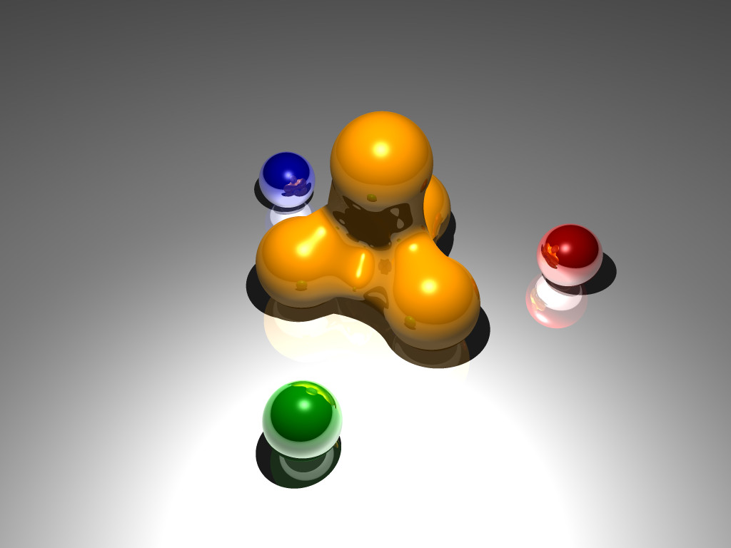
The second-last assignment in that class is to write a simple raytracer, using python to describe scenes which are thereafter rendered by a C/C++ back-end.  Once the basic requirements are met - simple lighting, shadows, scene hierarchies, etc. are working - students are free to add three (or more) features of their own accord.  I chose to add supersampling, reflections, and isosurface (blob) rendering using a simple solver.  Here are a few sample images.

The course-required images are somewhat less... erotic:

Moire Effect (1999)

In 1999, when starting university, I was still operating on somewhat older hardware (a pentium 133 and a 486/66, where most roommates had 400-500 MHz machines).  This being as it was, there were still a number of interesting demoscene effects I hadn't written up for myself, and I was still interested in learning about them.  On a rainy afternoon I tried my hand at writing a moiré effect.

The technique is pretty simple: a giant sprite is precomputed where the value of the color of a pixel is the radius from the center of the sprite, times a scalar constant to control radius, mod 32.  This yields a picture whose colour values consist of concentric rings with values increasing from 0 to 31, then 0 through 31 again, etc.  The palette is configured to consist of a gradient from black to white in colors 0 through 15, then white back to black in 16 to 31, so a single copy of the sprite rendered to the screen essentially looks like a series of concentric blurry circles.

At runtime, two copies of this sprite are offset in a simple moving pattern, and they are XORed into the framebuffer.  The XOR operation always a yields a value between 0 and 31, keeping the resulting colors in the frame buffer within the range of the preconfigured palette.  This yields the pattern which can be seen in the following movie.

Forging a Ring (2004)

In January 2004 I took a one-day blacksmithing course with some friends from UW engineering, which was great fun.  We essentially drove out to the boonies in the dead of winter, and spent our day huddled around forges in a real workshop.

We spent the morning learning the basics and forging hooks.  I'm not sure I recall the terminology, but we learned how to forge a flat tail (looks like a beaver tail), a pointy end (looks like a stabby weapon type of implement), and how to twist the rod.  This last operation was the most satisfying; you stick one end of the rod in a vise, and using a giant two-handed lever that threads around the square section of iron, you basically literally twist the metal with your bare strength after heating up the central section.  You even get to see little bits of colder metal flake of the twisting sections as you pull, which is very gratifying for the ego.

During the afternoon, we got around to forging iron rings.  (I had yet to see a true engineering iron ring at that point in my life, so my ring doesn't really look like the real thing.)  The teacher mag-welded our rings for us, and we polished them afterwards.

Mana - OpenGL Desktop (2002)

In 1995, I volunteered at a summer computer camp where the director worked on a NeXT machine.  I caught a glimpse of NeXTSTEP, and as a teen, the thing which impressed me with the machine and OS was the fact that on the desktop, a sphere continuously bounced back and forth across the screen.  That was it; a bouncing, rotating 3D sphere.  But it ran all the time, and it screamed "this machine is so powerful we can afford to waste cycles on useless, 3D background animations."  Keep in mind that 3D was just barely starting to make the rounds on consumer hardware at that point; SGI workstations were still very powerful (and expensive).

Fast-forward to 2002, when I began working as an intern for EA Canada, in Burnaby, BC.  We had dual-CPU machines, but very little software took advantage of this situation.  Even Visual Studio didn't support parallel builds yet.  (Note that much of our code was still built with 6.0.)  Because of this, it was mostly up to the OS to schedule entire programs to run in parallel.  However, though I did occasionally run two or more CPU-intensive programs at once (like, say, a data build along with a program compilation), this was definitely not a permanent state of affairs, which meant I basically had a processor sitting idle the vast majority of the time.

The NeXTSTEP background came to mind, and I figured something similar would be a nice way to harness that extra CPU power.  With a bit of idle time, I wrote a small app that creates a permanently-bottommost window and turns it into an OpenGL surface.  Ten years later, this actually still works on Windows 7 and looks even cooler with Aero, because of the window transparency effects.  However, it causes my computer's CPU fans to spin up because the cores are kept active and running at maximum frequency to handle the one busy thread (along with whatever work it dispatches to the graphics driver).

The "cool" part was actually figuring out how to make the window behave as a desktop.  Once I had that, I had to come up with something to render that wouldn't be too distracting, so I settled on a simple Sierpinsky pyramid (also apparently known as a tetrix, thank you wikipedia).  A few months later I also wrote a simple snow simulator because British Columbia is pretty green compared to Quebec, and I missed the weather from home.  It looks better at low resolutions but here goes anyway.

Quick and Dirty Q3A Level Viewer (2001)

In 2001, because of a bet of sorts with some friends, I spent the Canada Day evening and night trying my hand at writing a very simple Quake 3 Arena level viewer.  The morning after, I had basic walls, lightmaps, and broken static meshes rendering; I spent a bit more time that evening fixing the meshes' appearance, and came back a few days later to briefly look into curved surfaces (patches) for curiosity's sake.

I did not reverse-engineer the data format myself; I merely based my code upon Kekoa Proudfoot's excellent documentation.

Though this was really just a one-night, one-file experiment/hack that was never really meant to go anywhere, the results are visually amusing, so I thought I'd post a short video.  The orange "mystery" texture is where either I failed to export some textures by hand, or where the code discards materials because of over-complexity (I did not dive into supporting the material/shader system).

3D Fractal Pendulum (2001)

In university, in one of our calculus classes, we wound up briefly discussing numerical integrators and such.  Meaning to construct a playground to tinker with various integration schemes, I wound up writing an app which has pretty much nothing to do with the original intended purpose... but hey, since that's frequently where the most fun is found, I thought I would write a blurb about it anyway.

It's basically a simple 3D fractal, a kind of perfectly symmetrical, recursive pendulum.  It is effectively a visual representation of a binary tree; every node in the tree is represented by the intersection of two tubular segments.  It's fascinating to note that when tubular segment length is halved at each level of the hierarchy in the below video, none of the segments ever collide; in fact, they don't even come close.

Lego Mindstorms 3D Scanner / Virtual Inflater (2001)

In 2001, I purchased a second set of classic Lego Mindstorms from a coworker. Additionally, since I lived close to the St. Jacob's Lego Factory Outlet, I had purchased a bunch of extra parts that really made it possible to build really interesting projects. I decided to build a 3D rudimentary scanner using Lego; in 2001 this field had still not been explored very deeply by hobbyists, and I thought the challenge would be interesting.

Over a couple weeks I built a scanner, wrote driver software, and wrote mesh-reconstruction software to make use of the collected data. I initially tested the mesh-reconstruction software using synthesized data sets. When came the time to use the software with a real data set, I noticed that there seemed to be a small bug in the way the data was collected or transferred back the the computer... and believe it or not, I actually never spent the time to look into it. The robot wound up collecting dust for a couple of months before I recycled its parts for another creation. In hindsight, this is a huge regret for me since it was 99.5% there.

The idea behind the scanner is actually quite simple.  An object is placed on a rotating platter.  A light beam is swept back and forth across the object to capture a kind of 2D outline, as determined by the locations where the light beam is obstructed by the object.  The object is rotated to capture a series of 2D outlines, and software thereafter collates all that data into a final 3D mesh.

The Hardware

Though the robot itself was actually relatively simple, the 3-sensor limit on each RCX meant I had to make creative use of inputs.  (Keep in mind this was well before the NXT Mindstorms, and motors did not have positional feedback.)  Unfortunately, I do not have pictures of this robot - I owned no camera at the time.  However, I've modeled a crude Sketchup version which I hope gets the point across:

Degrees of freedom on the scanner.

The light beam was sent from one of the light sensors (in purple) straight into the other's receiver.  The LEDs in the RCX light sensors had a relatively tightly-focused light emission cone, so this worked quite well.

The teal assembly was rigid, and it moved vertically along the green assembly; the green assembly itself moved back and forth on the red horizonal axis.  Finally, the blue platter rotated on itself.

Robot Control

Two RCXs controlled the whole assembly:

Scanner system diagram.  (Click to enlarge.)

One RCX controlled the platter (in blue above) and collected the light beam data. The platter was quite simple; a motor slowly rotated the platter, and at preset angles, a touch sensor would be activated to tell the RCX to immobilize the platform. This was achieved using gear demultiplication; an offset nub on a "sensor gear" would trigger the sensor every time the sensor gear performed a full rotation. This sensor gear was configured to rotate sixteen times faster than the platter, thus yielding sixteen sensor touches per platter revolution, at equal intervals.

The other RCX was in charge of horizontal and vertical travel. One motor moved the light beam assembly horizontally, and had touch sensors at either end to detect the end of travel.  On the above diagrams, this is depicted as a red beam with a yellow sensor at either end.

The vertical axis (the green beam on the above diagrams) only had one sensor (depicted as another yellow block), at the top. During a scan run, the light beam assembly would start at the bottom and slowly make its way to the top. At the end of the scan run, it was returned to the bottom by shortly powering the motor to give the whole assembly downwards velocity, and then "floating" the motor to let the light beam assembly slowly return to the bottom of the vertical axis by pull of gravity. The assembly would come to a natural rest at the end of travel.

The RCXs were driven directly from Visual Basic code by talking to SPIRIT.OCX, the COM control used to interact with RCX bricks. At the time, VB was the easiest language to use when talking to the Spirit control, and since robot control and data collection task was not incredibly complex, VB was well-suited for the job.

One complication arising from the use of two RCXs was the fact that only one instance of SPIRIT.OCX could be loaded up per process space on Windows, and each Spirit control can only talk to a single RCX brick. To get around this limitation, I wrote two VB applications, each talking to its own Spirit control and underlying RCX.  The applications communicated over TCP/IP.

Data Collection

During a scan run, the robot would scan horizontal "slices" of the object, one at a time. To this end, it would
do the following:

• "Home" the robot, i.e. send it to a known starting state: reset the horizontal axis to one end, the vertical axis to the bottom, and the the platter to the next 1/16 revolution stop.
• For each slice:
• For each platter revolution stop:
• Travel the horizontal axis from one end to the other, and read light sensor levels at regular intervals.
• Rotate the platter to the next revolution stop.
• Travel the vertical axis up by a set distance.

The infrared ports between the RCXs and the computers were not quite speedy enough to stream the collected light levels back in real-time as the light beam assembly travelled horizontally. Thus, data was collected to the RCX's internal "datalog" memory, and after each horizontal axis travel was completed, the data was dumped back to the PC in bulk over infrared.

The Mesh-Reconstruction Software

The software which reconstructs the 3D mesh from the collected data operates in a number of discrete steps using a straighforward brute-force approach.  For the sake of example, let us assume we've scanned a short can-like object:

A short can.

Assume the can was resting upright when the scanner operated.  This yields a series of horizontal slices, taken in the same plane as the top and bottom of the can.

The same, with slices overlaid.

Let's focus on the top slice, the top of the can.  (The slice is not shaded the same as above because the generated normals do not match.)

A slice containing the top of the can.

As the scanner sweeps across the scanned shape, it collects a series of light levels at regular physical intervals.  These light levels are analysed using very simple statistical methods to determine where the object occludes the light, and where it does not.  (Note that the below is not representative of light readings for the above slice; it represents a run where the beam is blocked in two places, whereas for the convex slice above, the beam is only blocked in one place during the sweep.)

Light level readings and how object presence is determined. 

For a given sweep across the object, this gives us some notion of the object's profile along that axis, at the current slice's height.  To visualize this, let's view this slice from above:

The geometry which we are trying to extract.

To see how this geometry is constructed by the software, let's examine the algorithm conceptually, step by step. For example, for a single sweep, as seen from above (directly overhead), we might obtain the following edges:

Edges and projected volume for a single sweep.

On the above image, the robot detected light boundaries where the red lines are. The darker red area represents the area where where the object blocked the light. We know the object's profile must somehow fit within this region.

By rotating the platter on which the object rests, the robot can record multiple sweeps from a series of angles around the object, to see how the object's profile varies along with angle. This gives us very interesting data: specifically, we have snapshots of the volume the object must occupy from a number of differing projection incidence angles. For example, adding a second sweep:

Adding a second sweep.

The scanner this time found that the object occupied some area within the darkly-shaded green. Adding a third sweep:

...and a third sweep.

This is starting to get interesting. You can see that the intersection of the three shaded areas, in the middle, is starting to look like a circle. When you add the full series of sweeps and compute the intersection of all occlusion areas, you get the following:

All sweeps together.

How does the software compute the intersection, concretely?  In simple brute-force fashion; nothing better is really required for such small datasets, and the approach is easily debugged.  It begins by computing all intersection points between all edge pairs using simple 2D line-line intersections:

Computation of possible vertex set.

The next step discards all intersections which lie outside any given occlusion edge pair, i.e. outside any of the shaded areas in the previous diagrams.  If we know light flowed through a point from any angle around the object, it means that point cannot be inside the object.  After one discarding step:

Discarding vertices.

After two:

Discarding more vertices.

Note how the set of remaining vertices is pared down:

Remaining vertices part-way through discarding.

Keep going all around, and you are left with the following set of vertices:

Good vertices.

The program then trivially generates an edge loop and triangle fan to fit the resulting volume:

Edge loop.

Resulting triangle fan geometry.

This occurs for all slices of the object, with only the final geometry generation step being slightly more complex:

Light boundaries for all slices.

All intersections.

Good intersections.

Edge loops.

Resulting geometry; strips between slices, fans for the caps.

Normals, for lighting.  Lengths look bizarre, I know, not sure what that code was doing...  seems like it summed but did not divide to obtain an average among faces incident to a vertex.

There is not much more than that to it.  There is actually one more step that doesn't really show in the above, because the object does not contain holes.  If you scan an object like, say, this:

Object with a hole.

Then there is trickiness involved, because some slices will contain more than one closed area:

Edge loops on an object with a hole.

Mesh generation is solved by computing connectivity information from slice to slice.  There is a somewhat complex heuristic that attempts to determine how the centroids of various regions on neighbouring slices should be linked:

Region connectivity information (in teal).

Note that this will not give perfect results - we are essentially extrapolating spatial information that's missing between slices - but the idea is to gather a sufficient number of slices to make sure the error is not too large.

As I was writing this up (11 years later, in 2012), I thought it would be fun to generate some new, much more complex data and see how the inflater performs.  I wrote a small Sketchup plugin that essentially moves the camera around virtually as though it were the scanner head; at each location where a sample is taken, built-in Sketchup picking routines are used to determine whether anything blocks the camera's line of sight straight ahead.  I scanned the duck from the above renderings.  The duck is from the Sketchup model warehouse:

Virtually-scanned duck.

The result of a 96-slice, 32 angle-per-slice, 64 sample-per-angle scan is this mitigated result:

I wish I could zoom, but the executable contains no such feature, heh.  The triangle geometry looks really bad, but the edge loops actually look pretty decent.  This makes me happy, because going from raw light levels to edge loops was conceptually trickier than going from edge loops to geometry - there are number of known ways to do the latter reliably and robustly.

Edge loops.

(We can see a few artifacts in the form of "tunnels" crossing certain slices.  This is because my plugin script was a quick and dirty hack that doesn't handle all cases when dealing with data returned from Sketchup's picking routines.)