Mana - OpenGL Desktop (2002)

In 1995, I volunteered at a summer computer camp where the director worked on a NeXT machine.  I caught a glimpse of NeXTSTEP, and as a teen, the thing which impressed me with the machine and OS was the fact that on the desktop, a sphere continuously bounced back and forth across the screen.  That was it; a bouncing, rotating 3D sphere.  But it ran all the time, and it screamed "this machine is so powerful we can afford to waste cycles on useless, 3D background animations."  Keep in mind that 3D was just barely starting to make the rounds on consumer hardware at that point; SGI workstations were still very powerful (and expensive).

Fast-forward to 2002, when I began working as an intern for EA Canada, in Burnaby, BC.  We had dual-CPU machines, but very little software took advantage of this situation.  Even Visual Studio didn't support parallel builds yet.  (Note that much of our code was still built with 6.0.)  Because of this, it was mostly up to the OS to schedule entire programs to run in parallel.  However, though I did occasionally run two or more CPU-intensive programs at once (like, say, a data build along with a program compilation), this was definitely not a permanent state of affairs, which meant I basically had a processor sitting idle the vast majority of the time.

The NeXTSTEP background came to mind, and I figured something similar would be a nice way to harness that extra CPU power.  With a bit of idle time, I wrote a small app that creates a permanently-bottommost window and turns it into an OpenGL surface.  Ten years later, this actually still works on Windows 7 and looks even cooler with Aero, because of the window transparency effects.  However, it causes my computer's CPU fans to spin up because the cores are kept active and running at maximum frequency to handle the one busy thread (along with whatever work it dispatches to the graphics driver).

The "cool" part was actually figuring out how to make the window behave as a desktop.  Once I had that, I had to come up with something to render that wouldn't be too distracting, so I settled on a simple Sierpinsky pyramid (also apparently known as a tetrix, thank you wikipedia).  A few months later I also wrote a simple snow simulator because British Columbia is pretty green compared to Quebec, and I missed the weather from home.  It looks better at low resolutions but here goes anyway.

Refractive Lens Effect (1998)

In the '90s I really dug the demoscene.  Though I was never able to attend any parties, I would max out my BBS download quotas on all the demos I could lay my hands on.  Demos were always an inspiration to get better at coding, and learn about PC hardware.

In 1998, on a rainy afternoon, I decided to try my hand at writing a refractive lens effect somewhat like the one found in the Future Crew's Second Reality.  By now the demo had been out (and imitated) for many years, but hey, I was still working on the same 486, so better late than never.  (In a great twist of fate, I later wound up working at EA Montreal with a member of the Future Crew.)

The effect is very simple; a table of pointer offsets is precomputed, with one offset per pixel on the lens.  This table of pointer offsets can be thought of as being overlaid on top of the source image, at the lens position.  When rendering a given pixel on the lens, instead of a directly fetching the corresponding value in the source image, the precomputed offset is simply added to the raw address and the color value at that offset address is used instead.  For example, a precomputed offset of 1 will read the next pixel right; -1, the previous pixel, immediately to the left; 320, the next pixel down (since the screen is 320 pixels wide, with no padding/per-line stride); etc.  The offsets are precomputed to distort the source image as though it were being viewed through a refractive medium.

Hermite & Bézier Curve Testbed (1999)

When I first ran into the concept of parametric curves (thank you messirs Feiner, Hughes et al.), I wanted to write a small testbed to verify my understanding of the math.  It was a very simple application, written-just-before-supper type of thing, but I still find the simplicity of it to be pleasing... there's just something about the "straight pipedness" of mode 13h that will forever appeal to my senses.  :)

Quick and Dirty Q3A Level Viewer (2001)

In 2001, because of a bet of sorts with some friends, I spent the Canada Day evening and night trying my hand at writing a very simple Quake 3 Arena level viewer.  The morning after, I had basic walls, lightmaps, and broken static meshes rendering; I spent a bit more time that evening fixing the meshes' appearance, and came back a few days later to briefly look into curved surfaces (patches) for curiosity's sake.

I did not reverse-engineer the data format myself; I merely based my code upon Kekoa Proudfoot's excellent documentation.

Though this was really just a one-night, one-file experiment/hack that was never really meant to go anywhere, the results are visually amusing, so I thought I'd post a short video.  The orange "mystery" texture is where either I failed to export some textures by hand, or where the code discards materials because of over-complexity (I did not dive into supporting the material/shader system).

3D Fractal Pendulum (2001)

In university, in one of our calculus classes, we wound up briefly discussing numerical integrators and such.  Meaning to construct a playground to tinker with various integration schemes, I wound up writing an app which has pretty much nothing to do with the original intended purpose... but hey, since that's frequently where the most fun is found, I thought I would write a blurb about it anyway.

It's basically a simple 3D fractal, a kind of perfectly symmetrical, recursive pendulum.  It is effectively a visual representation of a binary tree; every node in the tree is represented by the intersection of two tubular segments.  It's fascinating to note that when tubular segment length is halved at each level of the hierarchy in the below video, none of the segments ever collide; in fact, they don't even come close.

E (1996)

Around 15 years of age I had a friend who also wanted to make games for a living.  We alternated between writing the required tools to create assets, and writing games themselves.

E (for editor) was the first somewhat serious graphical editor I decided to write.  I did so on and off in 1996,  over the course of a few weeks.  It was meant to work with the fixed palette I used within my video libraries, which essentially used 216 colors (6 possible color depths for each of red, green, and blue), along with a transparency key.  It supported the following features (more or less going off memory and a few minutes using it again to record the following video):

• individual pixel drawing, lines, rectangles, and ovals (no fill - that would come in a later iteration of the program)
• many methods to pick colors:
• a full-screen palette
• a mini-palette (full green-blue spectrum for a given red value)
• red-green-blue level pickers
• smooth shading gradient swatches; the user set either end of a gradient and the editor computed the intermediate colors
• a console to enter commands (file-related, tool selection, running effects, etc.)
• rectangular area selection
• many effects like blurring, sharpening, adding noise, tinting, etc.
• a snazzy windowing system

Lego Mindstorms 3D Scanner / Virtual Inflater (2001)

In 2001, I purchased a second set of classic Lego Mindstorms from a coworker. Additionally, since I lived close to the St. Jacob's Lego Factory Outlet, I had purchased a bunch of extra parts that really made it possible to build really interesting projects. I decided to build a 3D rudimentary scanner using Lego; in 2001 this field had still not been explored very deeply by hobbyists, and I thought the challenge would be interesting.

Over a couple weeks I built a scanner, wrote driver software, and wrote mesh-reconstruction software to make use of the collected data. I initially tested the mesh-reconstruction software using synthesized data sets. When came the time to use the software with a real data set, I noticed that there seemed to be a small bug in the way the data was collected or transferred back the the computer... and believe it or not, I actually never spent the time to look into it. The robot wound up collecting dust for a couple of months before I recycled its parts for another creation. In hindsight, this is a huge regret for me since it was 99.5% there.

The idea behind the scanner is actually quite simple.  An object is placed on a rotating platter.  A light beam is swept back and forth across the object to capture a kind of 2D outline, as determined by the locations where the light beam is obstructed by the object.  The object is rotated to capture a series of 2D outlines, and software thereafter collates all that data into a final 3D mesh.

The Hardware

Though the robot itself was actually relatively simple, the 3-sensor limit on each RCX meant I had to make creative use of inputs.  (Keep in mind this was well before the NXT Mindstorms, and motors did not have positional feedback.)  Unfortunately, I do not have pictures of this robot - I owned no camera at the time.  However, I've modeled a crude Sketchup version which I hope gets the point across:

Degrees of freedom on the scanner.

The light beam was sent from one of the light sensors (in purple) straight into the other's receiver.  The LEDs in the RCX light sensors had a relatively tightly-focused light emission cone, so this worked quite well.

The teal assembly was rigid, and it moved vertically along the green assembly; the green assembly itself moved back and forth on the red horizonal axis.  Finally, the blue platter rotated on itself.

Robot Control

Two RCXs controlled the whole assembly:

Scanner system diagram.  (Click to enlarge.)

One RCX controlled the platter (in blue above) and collected the light beam data. The platter was quite simple; a motor slowly rotated the platter, and at preset angles, a touch sensor would be activated to tell the RCX to immobilize the platform. This was achieved using gear demultiplication; an offset nub on a "sensor gear" would trigger the sensor every time the sensor gear performed a full rotation. This sensor gear was configured to rotate sixteen times faster than the platter, thus yielding sixteen sensor touches per platter revolution, at equal intervals.

The other RCX was in charge of horizontal and vertical travel. One motor moved the light beam assembly horizontally, and had touch sensors at either end to detect the end of travel.  On the above diagrams, this is depicted as a red beam with a yellow sensor at either end.

The vertical axis (the green beam on the above diagrams) only had one sensor (depicted as another yellow block), at the top. During a scan run, the light beam assembly would start at the bottom and slowly make its way to the top. At the end of the scan run, it was returned to the bottom by shortly powering the motor to give the whole assembly downwards velocity, and then "floating" the motor to let the light beam assembly slowly return to the bottom of the vertical axis by pull of gravity. The assembly would come to a natural rest at the end of travel.

The RCXs were driven directly from Visual Basic code by talking to SPIRIT.OCX, the COM control used to interact with RCX bricks. At the time, VB was the easiest language to use when talking to the Spirit control, and since robot control and data collection task was not incredibly complex, VB was well-suited for the job.

One complication arising from the use of two RCXs was the fact that only one instance of SPIRIT.OCX could be loaded up per process space on Windows, and each Spirit control can only talk to a single RCX brick. To get around this limitation, I wrote two VB applications, each talking to its own Spirit control and underlying RCX.  The applications communicated over TCP/IP.

Data Collection

During a scan run, the robot would scan horizontal "slices" of the object, one at a time. To this end, it would
do the following:

• "Home" the robot, i.e. send it to a known starting state: reset the horizontal axis to one end, the vertical axis to the bottom, and the the platter to the next 1/16 revolution stop.
• For each slice:
• For each platter revolution stop:
• Travel the horizontal axis from one end to the other, and read light sensor levels at regular intervals.
• Rotate the platter to the next revolution stop.
• Travel the vertical axis up by a set distance.

The infrared ports between the RCXs and the computers were not quite speedy enough to stream the collected light levels back in real-time as the light beam assembly travelled horizontally. Thus, data was collected to the RCX's internal "datalog" memory, and after each horizontal axis travel was completed, the data was dumped back to the PC in bulk over infrared.

The Mesh-Reconstruction Software

The software which reconstructs the 3D mesh from the collected data operates in a number of discrete steps using a straighforward brute-force approach.  For the sake of example, let us assume we've scanned a short can-like object:

A short can.

Assume the can was resting upright when the scanner operated.  This yields a series of horizontal slices, taken in the same plane as the top and bottom of the can.

The same, with slices overlaid.

Let's focus on the top slice, the top of the can.  (The slice is not shaded the same as above because the generated normals do not match.)

A slice containing the top of the can.

As the scanner sweeps across the scanned shape, it collects a series of light levels at regular physical intervals.  These light levels are analysed using very simple statistical methods to determine where the object occludes the light, and where it does not.  (Note that the below is not representative of light readings for the above slice; it represents a run where the beam is blocked in two places, whereas for the convex slice above, the beam is only blocked in one place during the sweep.)

Light level readings and how object presence is determined. 

For a given sweep across the object, this gives us some notion of the object's profile along that axis, at the current slice's height.  To visualize this, let's view this slice from above:

The geometry which we are trying to extract.

To see how this geometry is constructed by the software, let's examine the algorithm conceptually, step by step. For example, for a single sweep, as seen from above (directly overhead), we might obtain the following edges:

Edges and projected volume for a single sweep.

On the above image, the robot detected light boundaries where the red lines are. The darker red area represents the area where where the object blocked the light. We know the object's profile must somehow fit within this region.

By rotating the platter on which the object rests, the robot can record multiple sweeps from a series of angles around the object, to see how the object's profile varies along with angle. This gives us very interesting data: specifically, we have snapshots of the volume the object must occupy from a number of differing projection incidence angles. For example, adding a second sweep:

Adding a second sweep.

The scanner this time found that the object occupied some area within the darkly-shaded green. Adding a third sweep:

...and a third sweep.

This is starting to get interesting. You can see that the intersection of the three shaded areas, in the middle, is starting to look like a circle. When you add the full series of sweeps and compute the intersection of all occlusion areas, you get the following:

All sweeps together.

How does the software compute the intersection, concretely?  In simple brute-force fashion; nothing better is really required for such small datasets, and the approach is easily debugged.  It begins by computing all intersection points between all edge pairs using simple 2D line-line intersections:

Computation of possible vertex set.

The next step discards all intersections which lie outside any given occlusion edge pair, i.e. outside any of the shaded areas in the previous diagrams.  If we know light flowed through a point from any angle around the object, it means that point cannot be inside the object.  After one discarding step:

Discarding vertices.

After two:

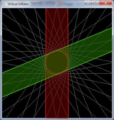Discarding more vertices.

Note how the set of remaining vertices is pared down:

Remaining vertices part-way through discarding.

Keep going all around, and you are left with the following set of vertices:

Good vertices.

The program then trivially generates an edge loop and triangle fan to fit the resulting volume:

Edge loop.

Resulting triangle fan geometry.

This occurs for all slices of the object, with only the final geometry generation step being slightly more complex:

Light boundaries for all slices.

All intersections.

Good intersections.

Edge loops.

Resulting geometry; strips between slices, fans for the caps.

Normals, for lighting.  Lengths look bizarre, I know, not sure what that code was doing...  seems like it summed but did not divide to obtain an average among faces incident to a vertex.

There is not much more than that to it.  There is actually one more step that doesn't really show in the above, because the object does not contain holes.  If you scan an object like, say, this:

Object with a hole.

Then there is trickiness involved, because some slices will contain more than one closed area:

Edge loops on an object with a hole.

Mesh generation is solved by computing connectivity information from slice to slice.  There is a somewhat complex heuristic that attempts to determine how the centroids of various regions on neighbouring slices should be linked:

Region connectivity information (in teal).

Note that this will not give perfect results - we are essentially extrapolating spatial information that's missing between slices - but the idea is to gather a sufficient number of slices to make sure the error is not too large.

As I was writing this up (11 years later, in 2012), I thought it would be fun to generate some new, much more complex data and see how the inflater performs.  I wrote a small Sketchup plugin that essentially moves the camera around virtually as though it were the scanner head; at each location where a sample is taken, built-in Sketchup picking routines are used to determine whether anything blocks the camera's line of sight straight ahead.  I scanned the duck from the above renderings.  The duck is from the Sketchup model warehouse:

Virtually-scanned duck.

The result of a 96-slice, 32 angle-per-slice, 64 sample-per-angle scan is this mitigated result:

I wish I could zoom, but the executable contains no such feature, heh.  The triangle geometry looks really bad, but the edge loops actually look pretty decent.  This makes me happy, because going from raw light levels to edge loops was conceptually trickier than going from edge loops to geometry - there are number of known ways to do the latter reliably and robustly.

Edge loops.

(We can see a few artifacts in the form of "tunnels" crossing certain slices.  This is because my plugin script was a quick and dirty hack that doesn't handle all cases when dealing with data returned from Sketchup's picking routines.)